Observation Parameters

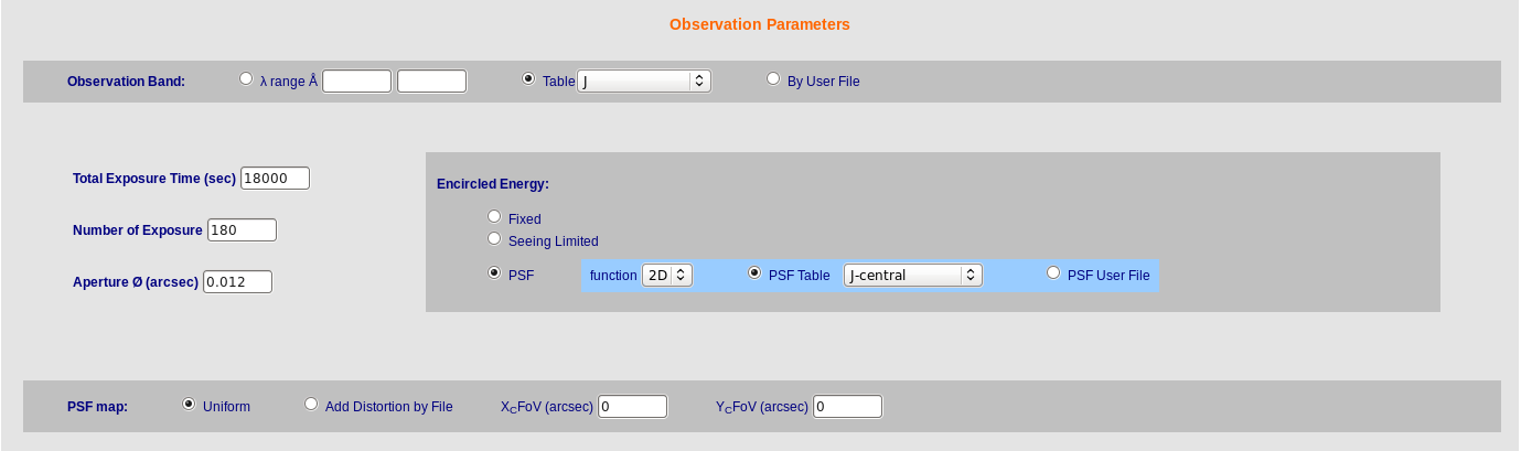
Observation band: Definition of the observation band. It is possible to select among these different choices:
- a fixed wavelength (λ) range: entering the start (λ₁) and end (λ₂) wavelengths in Å
- a passband from a filter list (Table)
- a defined user file with the passband giving wavelength (Å) and transmission [range 0.0 - 1.0];
  Below an example of observation band user file:
```
# Table : Filter.dat
# put comment character #, at the beginning of each comment line
# Wavelength  Transmission 
#  (A)       [0.0 - 1.0]
#
  4500 0.10
  5000 0.20
  5500 0.30
  6000 0.25
  7000 0.10
  8000 0.05
```
Total Exposure time: The total integration time of the observations in seconds.
Number of Exposures: Number of individual exposures to reach the total integration time.
Aperture: The diameter (in arcsec) of the circular aperture where the signal is integrated to compute the expected Signal-to Noise ratio.
Encircled Energy: The fraction of light that is collected within the Aperture.
The available options are:
- Fixed: A constant and fixed value must be inserted (in this case no definition of the PSF is required)
- Seeing limited: The PSF is assumed a Gauss or Moffat function of a given FWHM (in arcsec)
- PSF: The PSF profile can be defined as:
  - 1D radial intensity profile, selecting one of the available PSF tables or providing a configuration file with Radius (arcsec) and Intensity [0.-1.0], (see example below )
  - 2D image (as FITS file).
    In the option PSF Table a number of PSF images are available for MICADO@E-ELT (MAORY), WFPC2@HST, NIRcam@JWST. For user defined PSF image (PSF User File) a fits image is required with the PSF at the center of the fits image.
  - NOTE : if the PSF has a pixel scale different from the simulated image then the keyword PSFSCALE is required in the fits giving arcsec/pixel of the input PSF file.
  - 3D data-cube (as FITS file).
    For details about the 3D PSF see the Advanced Help.
  The Encircled Energy is then computed from the integrated flux inside the given aperture.
PSF map: In the case of 1D or 2D PSF, the input PSF can be either uniform or variable in the field of view:
- Uniform: A constant PSF in the whole simulated field of view
- Distortion file: Select this option to provide a distortion map.
  The PSF (as defined in the above configuration) is distorted depending on the position in the field. The distortion is provided by a table (ASCII file) giving a map of the distortion. The distortion map is a table yielding a list of positions in the field (defined by the pixel coordinates X, Y), the ratio between the size (FWHM-ratio) of the PSF in the X,Y position and the input PSF, the added distortion of shape given by the ellipticity of the PSF (between 0 and 1) and the position angle of the major axis of the elongated PSF in degrees counted anti-clockwise at the current position (X, Y). The PSF used for the simulated image is then computed at each coordinate by interpolating the nearest values from the distortion table. Here an example of PSF distortion file:
```
# Example of PSF distortion map :
#   X       Y    FWHM(ratio)   Ellipticity   Position_Angle
  100    100     0.72              0.32                -80
  200    100     0.79              0.24                -60
  300    100     0.86              0.16                -40
  400    100     0.93              0.08                -20
# ...
  100    400     0.72              0.32                -80
  200    400     0.79              0.24                -60
  300    400     0.86              0.16                -40
  400    400     0.93              0.08                -20
  500    400     1.00              0.00                  0
# .....
  500    700     1.00              0.00                  0
  600    700     1.07              0.08                 20
  700    700     1.14              0.16                 40
  800    700     1.21              0.24                 60
  900    700     1.28              0.32                 80
```